Most of us get our work done by collaborating and working in teams. Organizing and keeping up with all the assigned tasks, documents, and conversations related to a group’s work is often difficult because of all of the juggling one has to do to keep up with the flow of information and conversations. However, Google has made it much easier with an app called Spaces.
Enabling Spaces in Gmail
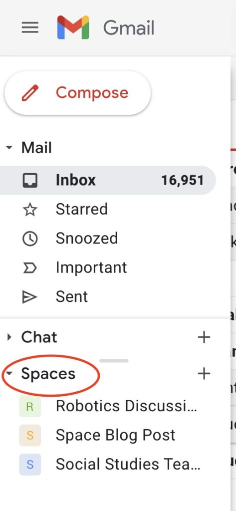
If a user has enabled the Chat feature in Gmail, you will notice that Spaces is located just below Chat. Spaces are available for both enterprise users (such as Google Workspace) and free accounts. If you don’t see it in your account, go to your settings (the gear icon), then click on “See all settings,” then on “Chat and Meet.” Make sure “Google Chat” is selected. It was turned on for my work account but not my personal account. As soon as I turned on Google Chat in my personal account, Spaces was immediately added.
Setting Up Spaces
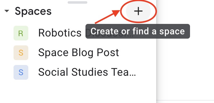
Spaces are located on the left-hand menu of your Gmail on a desktop. Click on the + sign to create a Space.
On your phone, the icon is located at the bottom of the screen. It’s the icon of a group of people.

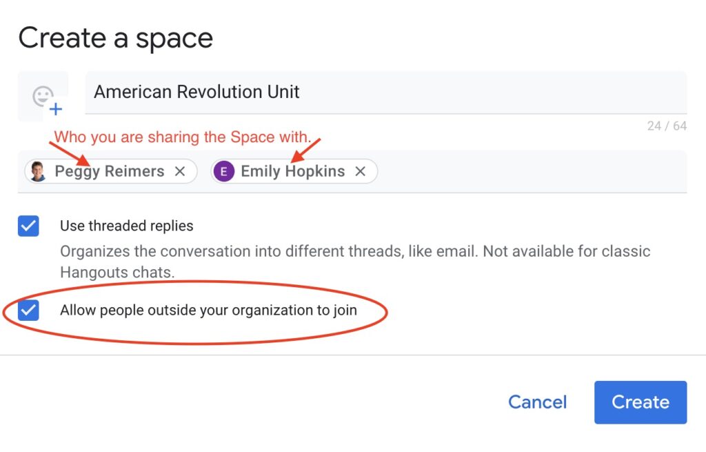
When you create a space, you will first need to name it. You will also add the different individuals that will work with you on this project. You will then need to decide if you want to allow people outside your organization to join the space. The choice to add people outside your organization is only available when you set up your space, so make sure you think this through when you create a space. You can’t add people outside your organization later if you don’t make this selection when you create the space.
Adding Files to Google Spaces
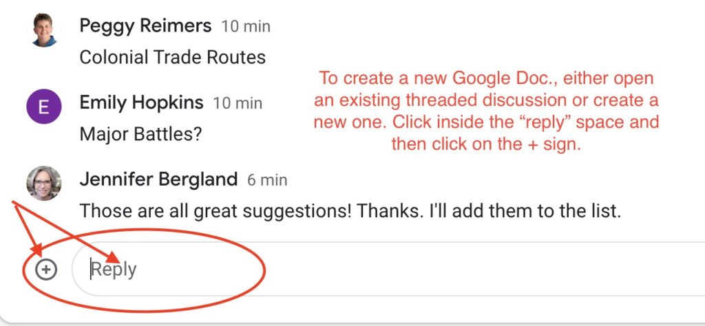
There are two ways you can add Google files to your space. You can add an existing file or create one within the space. If you want to create a file within the space, you must either open an existing threaded discussion or create a new one. You will then need to click in the space where you would compose a reply. That will make the + sign link active. Click on the + sign, and it will open up a dialogue box that lists the different types of Google docs. You will click on the type you want to create and proceed as normal.
Once the file is created, it will be within your space as well as in your Google Drive.
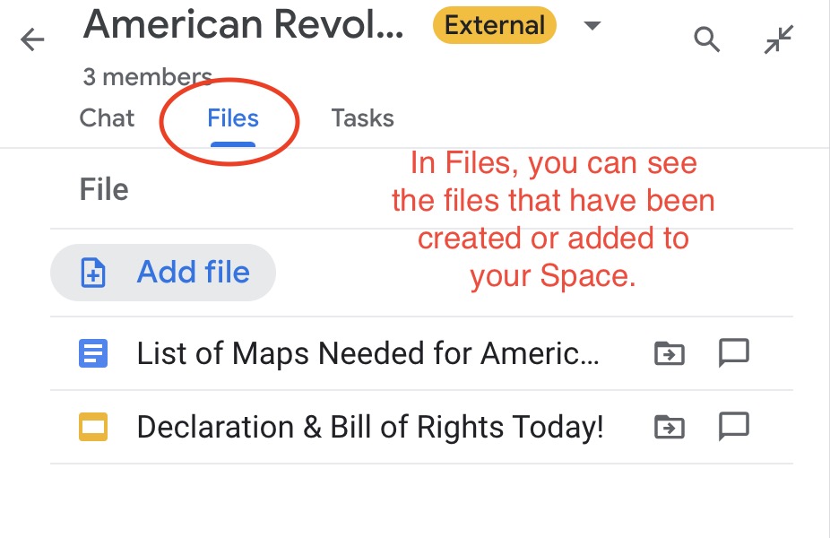
Activities Within Google Spaces App
Once you have created your space, you will also have the ability to add people, share files, and assign tasks.

Adding and Assigning Tasks
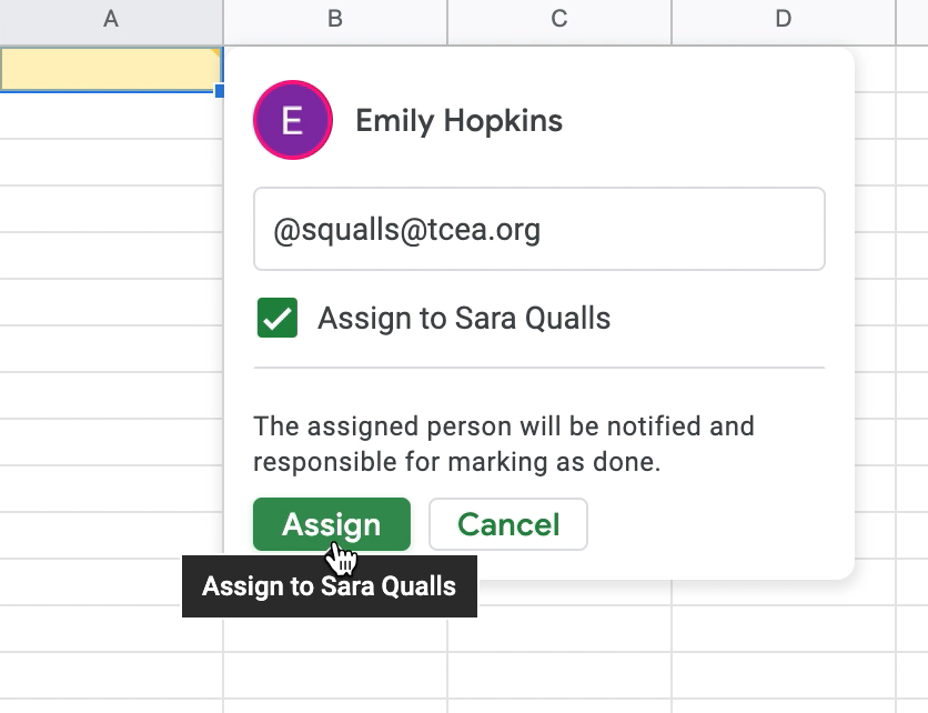
Adding tasks is where the power is. This is where you create the tasks that need to be accomplished.
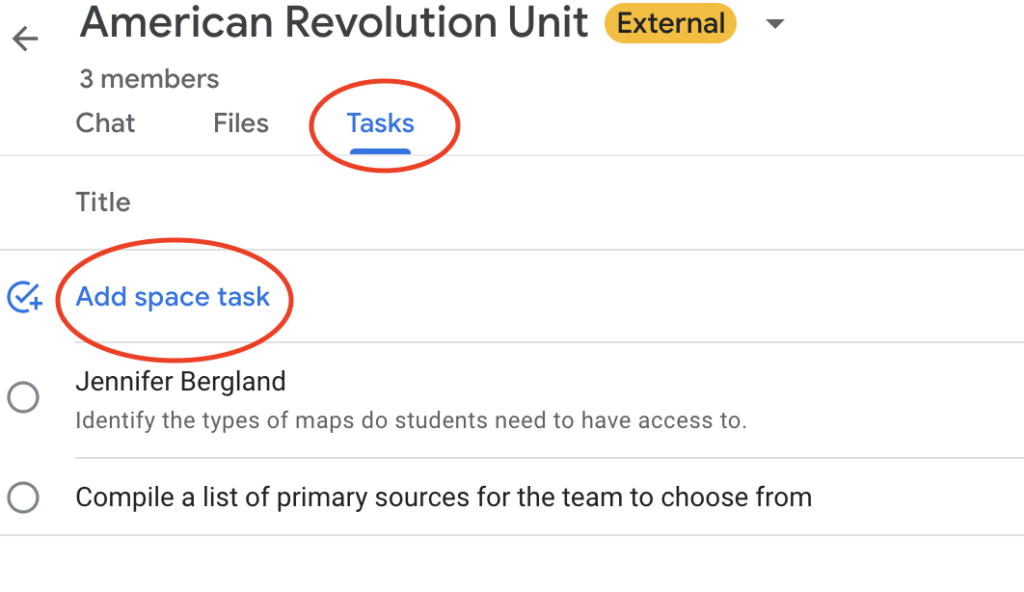
You can also determine when the tasks will be completed and by whom.


Searchability Within Google Spaces
One of the things that makes Google’s Spaces especially useful is searchability. It makes it easy to find tasks, discussions, and items that pertain to a specific topic or task.
This enhanced feature in Gmail can greatly enhance your work, especially when collaborating with others. This tool is useful for both teachers and administrators and for both short and long-term projects. Try it out, and let me know how it goes in the comments!

