

Struggling to take your Google Sheets beyond data collection and surveys? Do you think spreadsheets are only helpful when investigating trends within your classroom? While Google Sheets can provide you with ways of analyzing your data to impact your instruction, let’s explore five tricks that can take you far beyond those capabilities.
1. Conditional Formatting in Google Sheets
What if I’d like students’ responses to be automatically color-coded?
Conditional Formatting makes this process efficient and an absolute time saver. Google Sheets provides you with ways to automatically color code responses to provide that “instant check” of student work. This can apply to both text and numbers, depending on your need.
Use this skill to:
- Highlight student responses on a discussion board that contains a certain word or phrase.
- Check student solutions to a mathematics or science problem.
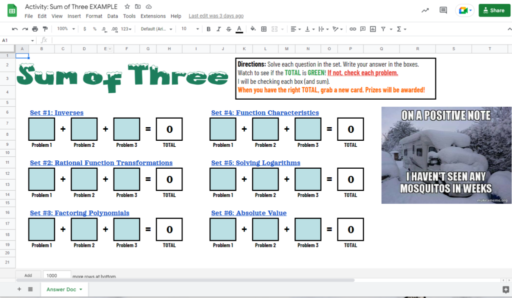
- Insert checkboxes as a way for students to monitor their progress through a blended learning unit. Checkboxes can turn green once selected by using “TEXT EQUALS TRUE” under the Conditional Formatting menu.
In the Algebra 2 example below, students solved three problems within a skill set and Google Sheets automatically checked if their total was correct. If it wasn’t, students needed to work through their problems again, encouraging error analysis conversations and academic collaboration. Learn how to get started with conditional formatting.
2. Data Validation
What if I want students to select a phrase or word from a dropdown menu?
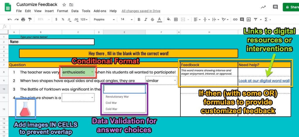
Data Validation, located under the Data menu, can help with this. You can create a specific list of items, i.e. answers, for students to select from to alleviate any spelling concerns. This is perfect for those fill-in-the-blank activities, sequencing events, geometric proofs, and student surveys. Use the date option instead to create a sign-up Google Sheet for student presentations, grade interviews, or small group instruction.
DID YOU KNOW: You can combine this skill with conditional formatting! Choose an answer and it can automatically go green. Check out this example to test it out.
3. IF Formulas in Google Sheets
What if I want students to get scaffolded support based on which answer they type?
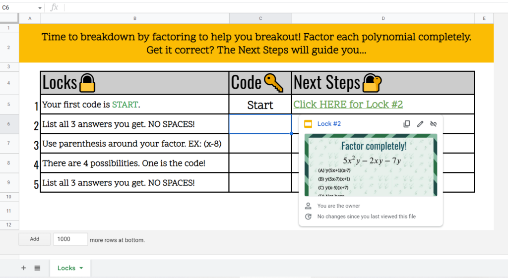
Using the IF formula, Google Sheets will check the student’s work against the correct answer that you provide, and then provide support with either text or a link to an external resource. You can even create digital breakout activities using the IF formula. For example, IF students type the code “MATH ROCKS”, THEN next clue is given. In general, your formula will look like:
=IF(Cell= “Code”, “Correct answer next steps”, “Wrong answer next steps/Feedback”)
=IF(C5=“Start”, “Congrats! Your next lock is…”, “Revisit our 2.1 notes.”)
Check out this Algebra 2 example where students practiced factoring polynomials. Learn how to get started with this digital breakout tutorial using Sheets and this TEMPLATE.
This Geometry example, created by Mandi Tolen, utilizes the same IF formula and conditional formatting to automatically have a hidden picture appear if students answer questions correctly. Learn and practice with her Google Sheets template on her blog post.
4. Hyperlinks
What if I want students to explore a website, watch a video, or reference a digital classroom material within an activity?
The Hyperlink formula will accomplish just that! Combine the Hyperlink formula with the IF formula to provide students with reteach pieces or interventions. Link to anchor chart images, online exploration exercises, or Slides with questions like the example above. In general, your formula will look like:
=hyperlink(“web URL address”, “title of the link”)
5. Google Sheets’ vLookup
Do you have a list of task cards that you’d like students to complete AND have their answers checked?
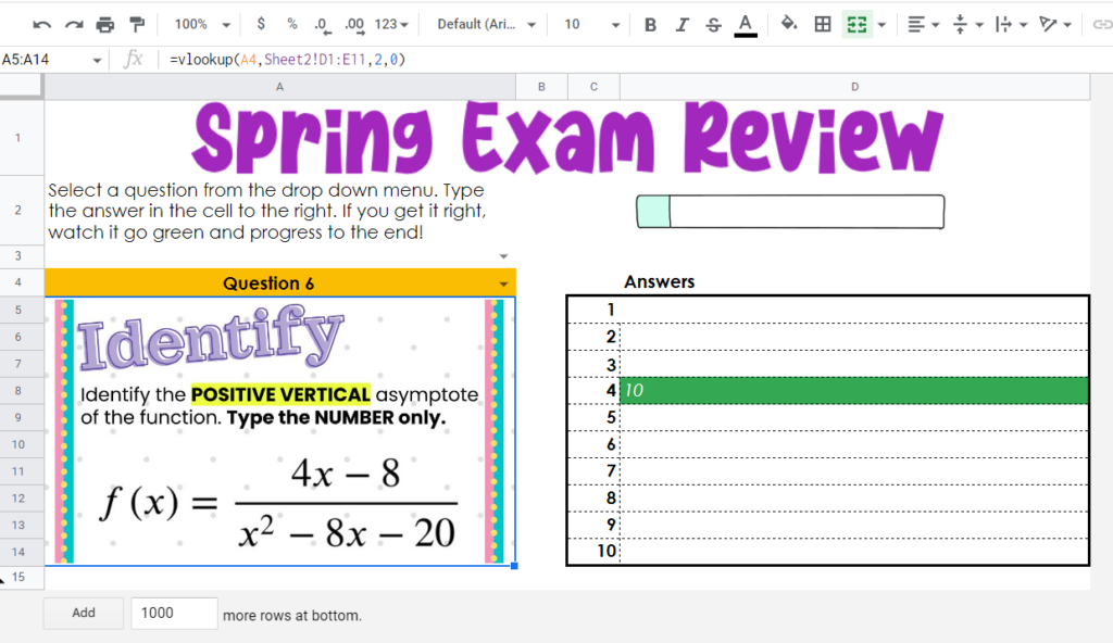
Use the VLOOKUP formula to pull in questions based on what students want to work on. This formula will take the students’ selection, vertically locate the task from a list you’ve created, and automatically pull it up for students. Combine this skill with conditional formatting in Google Sheets so that students’ answers can be checked while they work. Check out the Algebra 2 example below on characteristics of rational functions. This activity allowed students to work in any order within the ten provided questions. Take a look at this blog post from Mandi Tolen to learn more and snag a template.
I hope these five tricks help you leverage the power of Google Sheets to provide instant feedback and create engaging experiences for your students. Let’s take those worksheets and make them into authentic “work”sheets!
To learn more from Lauren, take a look at the sessions she’s leading at TCEA 2023, January 30- February 2 in San Antonio, TX. Want to be in the middle of some majorly innovative learning, meet other passionate educators, and explore limitless possibilities in ed tech? Early bird pricing ends November 4. Don’t miss it!