

Do you ever wish the color of your spreadsheet rows would change color to match the content? If yes, you may enjoy learning about conditional formatting. Conditional formatting is a wonderful feature in Google Sheets and Microsoft Excel. Let’s explore how to use custom formulas that can change the color of cells and rows of data based on the data in a cell.

Meet the Problem
“Oh, I use conditional formatting all the time. But I want to change the colors of the first column when the data in the last column changes. How could I do that?”
It might help to see what this problem looks like. Most spreadsheet users know you can use conditional formatting.
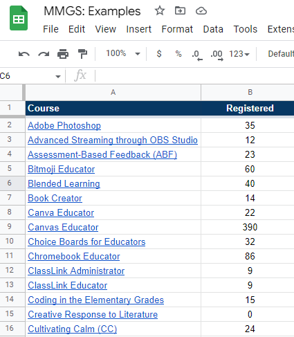
Consider this spreadsheet, which represents a list of workshops and the number of registrants for each course:
Conditional formatting could allow me to change the colors. For example, I could add conditional formatting rules for different conditions. Let’s take a look at examples.
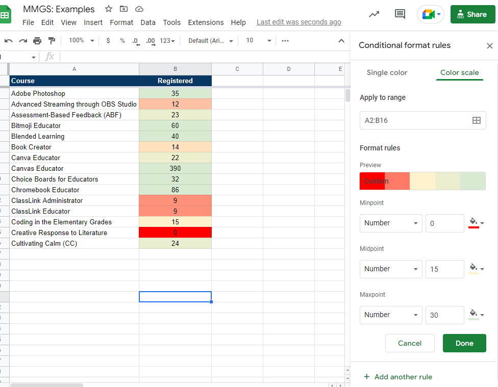
1) Create a sliding color scale.
These settings would adjust the colors of the cells where values appear. For example, the minimum number “0” would be red. The midpoint (“15”) would be yellow, and the maxpoint (“30”) would be green. You can see what that looks like below, as well as take a look at the color scale:
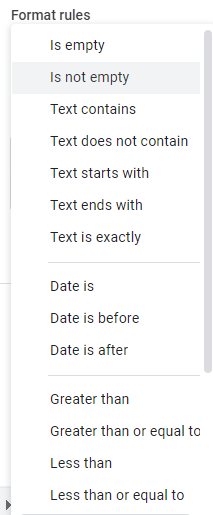
2) Apply single colors.
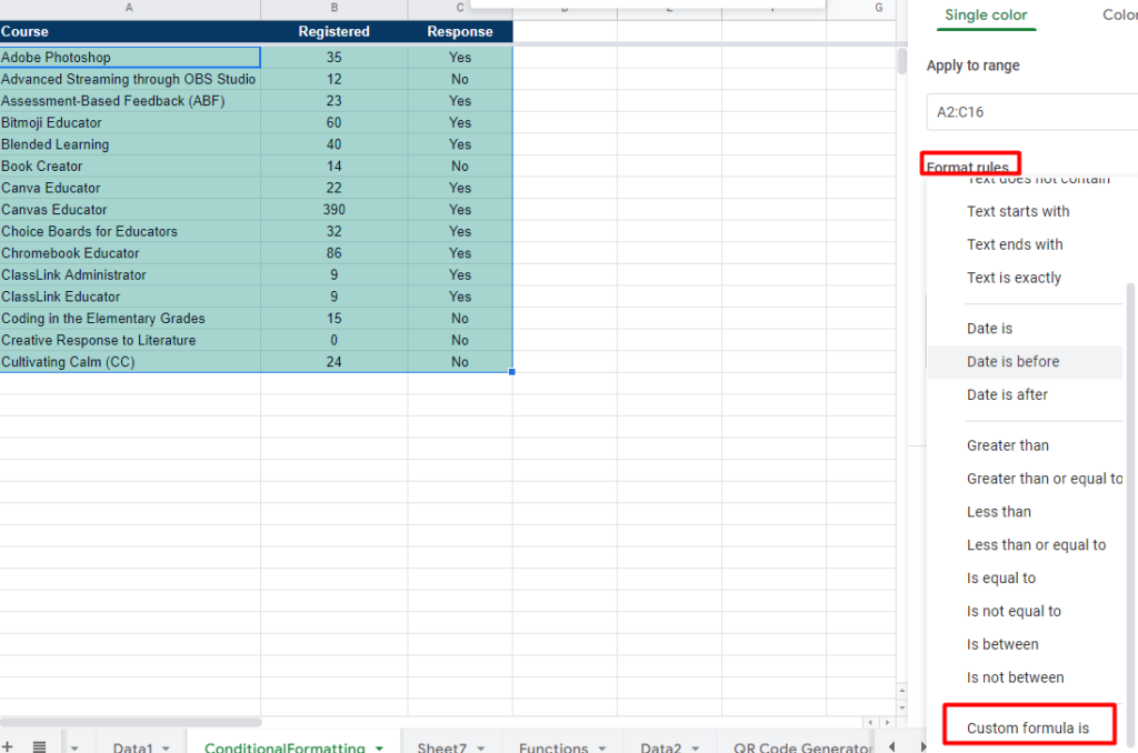
This is the most often used conditional formatting solution. In this case, you can use a variety of format rules. These format rules say, “Format cells if…” certain conditions are met. Here is the list of most conditions you can apply:
I often use these when getting data from a Google Form, and I want to see how YES or NO responses look.
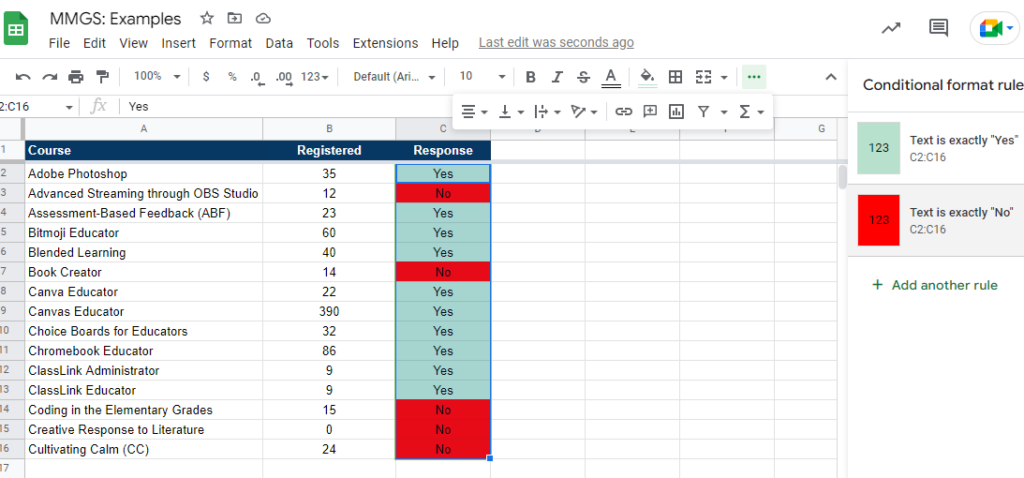
As you can see in the screenshot above, conditional formatting changes the color of the cell. The colors depend on the value in the cell. In this case, “Yes” is green, and “No” is red.
But what happens when you want the entire row to be green or red based on the YES or NO? That’s where custom formulas come to the rescue.
Introducing Custom Formula
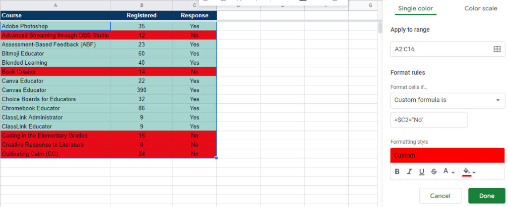
Custom formula makes it easy to apply colors and formatting to an entire row of data. After you highlight the rows you want to apply conditional formatting to, go to Format -> Conditional Formatting. Then, enter a formula into the “Custom Formula” option, as shown below:
You can see that you will need to enter a “value or formula” into the custom formula box:
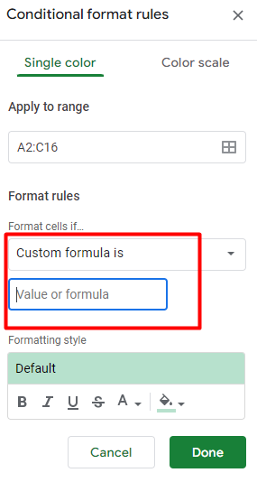
This will allow you to enter a formula for the conditional formatting rule. In this case, I want two rules to be present:
- When the word “Yes” appears in column “C,” the entire row to turns green
- When the word “No” appears in column “C,” the entire row to turns red
But how do you do that? What do you type into the custom formula box?
Here’s what that looks like with one custom formula rule applied:
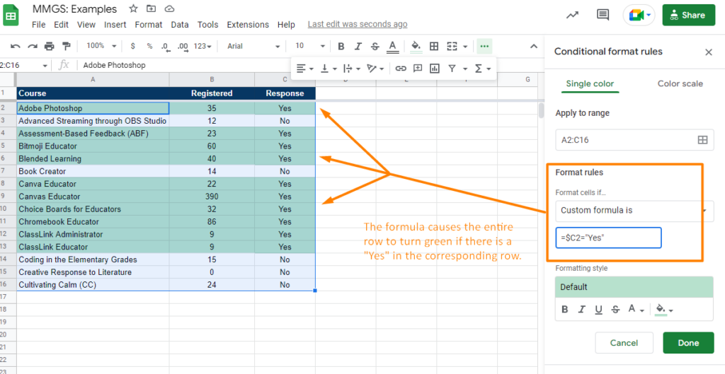
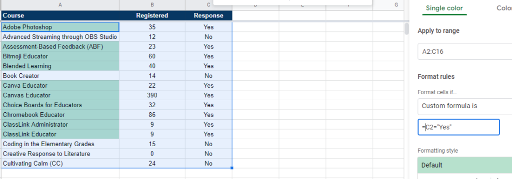
Notice that the $ in the formula applies formatting that matches the row of data where it appears (A2 to C2, A3 to C3). This is referred to as “absolute references” rather than relative references. If I were to not include the dollar sign, only the first column would change color, as you can see below:
To add the red fill color to each cell in a row, I have to add another rule:
Both of the custom formula rules appear below:
- When the word “Yes” appears in column “C,” the entire row to turns green: =$C2= “Yes”
- When the word “No” appears in column “C,” the entire row to turns red: =$C2= “No”
And that looks like this:
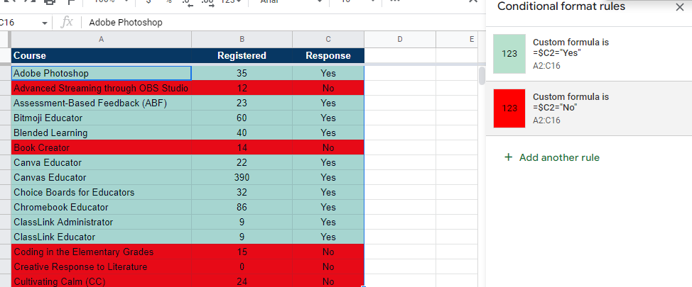
Isn’t that cool?
Want to Learn More?
As a Google Sheets user, I often find myself learning new things about stuff I thought I knew. I’ve been using conditional formatting for years. Yet, I never thought to scroll to the bottom of the formatting rules to see what else was there! Now that you know about custom formulas in conditional formatting, how will you use them?
Learn more about conditional formatting and Google Sheets:
- Microsoft Excel
If you don’t use either Google or Microsoft, give OnlyOffice a try. It also offers many features in spreadsheets without the price. You can read my blog entry about OnlyOffice here.